Understanding modelled economic evaluations: a reader's guide for clinicians

Economic evaluations have a long history in health care.1,2 Full economic evaluations aim to inform decision making through comparing the costs and outcomes of two or more interventions, strategies, programs or policies, to estimate their efficiency via an incremental cost‐effectiveness ratio. The premise for conducting economic evaluations is that health care resources are finite, and there is an opportunity cost when resources are allocated to one health care intervention over another.3,4 In Australia, economic evaluations are important considerations in policy decisions on what should be publicly funded under the Pharmaceutical Benefits Scheme (PBS)5 and Medicare Benefits Schedule (MBS).6 Furthermore, clinician–researchers are increasingly considering both clinical effectiveness and cost‐effectiveness in evaluation studies and funding applications.

Full economic evaluations are classified by the type of evaluation, with the most common types being cost‐effectiveness analysis (CEA), cost–utility analysis (CUA) and cost–benefit analysis (CBA).3 The method for conducting these economic evaluations can be study‐based or decision–analytic model‐based, or both.7 Modelled economic evaluations can overcome some of the limitations associated with study‐based economic evaluations.7,8 The complexity and use of modelled evaluations has increased with improved computing power and data availability. Several published articles offer clinicians an introduction to economic evaluations,1,9,10 but few to date have focused on modelled evaluations.11,12 In this key research skills article, we aim to improve clinician understanding of modelled evaluations. In the Supporting Information, we illustrate key modelling concepts using two recently published models in the Medical Journal of Australia.

Why modelled economic evaluations?

Why are model‐based evaluations done? Modelled evaluations can be performed alongside empiric studies or as standalone studies. Modelled evaluations do not replace study‐based evaluations — rather, they enable evidence synthesis across multiple studies into relevant decision‐making contexts, extrapolation of trial‐based results beyond the time horizon, and hypothesis generation where data are unavailable.7,8,13 Box 1 outlines key areas in which study‐based and model‐based economic evaluations differ.

We use an example of a randomised controlled trial (RCT) calculating the cost‐effectiveness of a new blood pressure medicine compared with placebo to illustrate why modelled evaluations might be required. Firstly, the model can be used to synthesise evidence across multiple trials for decision making.8 Whereas the RCT is only comparing the new medicine against the placebo, a modelled evaluation can extend this to compare the new medication against several commonly used blood pressure agents not included in the trial.

Secondly, models can extrapolate findings beyond the trial‐based follow‐up period (time horizon). If the above RCT was conducted over two years, the quality‐adjusted life years (QALYs; Box 2) gained through improved blood pressure management are likely to be accrued over an individual's lifetime (eg, long term reduction in cardiovascular events) rather than simply within the two‐year follow‐up period of the RCT. Therefore, the model can be used to extrapolate cost‐effectiveness to an appropriate time horizon.7

Thirdly, using cost‐effectiveness results from a single trial can be problematic if the trial is not generalisable to the population or health care setting in which the decision is being made.7 For example, if the RCT was done in the United States, a modelled evaluation can use Australian estimates of health care use and costs to assist with decision making on whether the new medication is cost‐effective in our local context.

Which models are used and why?

The type of decision–analytic model used depends on several factors, including the decision context, data availability, and interpretability of the model.15 Below we cover several common model types including simple decision trees, Markov cohort, and Markov microsimulation models. Box 3 summarises common terms used in modelled economic evaluation.

Simple decision tree

Consider a simple example of calculating the cost‐effectiveness of a new blood pressure medicine compared with placebo. A simple decision tree can be constructed with the one‐year probabilities of developing outcomes of cardiovascular disease (CVD) and death. In Box 4, the intervention cohort had a lower probability of developing CVD (15%) compared with the placebo cohort (25%). Costs and outcomes are calculated for both intervention and placebo groups (see example of how cost is calculated for the new blood pressure medicine in Box 4). From costs and outcomes, an incremental cost‐effectiveness ratio (ICER; Box 2) can be calculated, for example, $30 000 per QALY gained. The decision tree is easily interpretable but infrequently used because of inherent difficulties in incorporating longer term cost‐effectiveness.15

Markov cohort

Markov models are widely used to represent the movement between different health states over time.8 Box 5 shows a Markov cohort model for a similar scenario as described above. For simplicity, we assume that the annual probabilities of developing outcomes of CVD and death remain constant over 30 years. If we model a population of 100 patients in a Markov cohort model, the entire cohort enters and moves through the model for 30 years, at one‐year cycles. All patients have no CVD at the start, but by the end of Year 1, 15 (15% of 100 people) with no CVD develop CVD. Box 6 follows the cohort through Years 1 to 4. The ICER now reflects the differences between intervention and control groups over 30 years, rather than the one year as per the simple decision tree. To conduct the same analysis using a simple decision tree would require an additional branch for each of the 30 years modelled.

Markov microsimulation

For the same scenario as above, a Markov microsimulation model, also known as a first‐order Monte Carlo simulation, can be constructed. The structure of the model would be the same as the Markov cohort model (Box 5). However, in microsimulation, each of the 100 patients moves through the model individually until the end of 30 years. For example, in Box 6, Person 1 develops CVD in Year 4 (orange bubble), and the model follows this individual's journey over 30 years or until death. The simulation is repeated for each person until all 100 individuals complete their 30 years simulated disease journey. Microsimulation enables greater model complexity. For example, the probability of death for Person 1 can be changed to reflect their individual demographic profile (eg, age, sex), or their number of years living with CVD.8 Using microsimulation, cost‐effectiveness for subpopulations can be calculated separately — for example, separate ICER of new medicine versus placebo for male and female patients.

Discrete event simulation

Discrete event simulation (DES) is a microsimulation model where individuals move through health states according to time‐to‐event probability distributions. These are less commonly used in economic evaluations than above models, but may offer greater flexibility than Markov microsimulation, for example, in its treatment of time and handling of the simultaneous risk of multiple events.16,17

Model uncertainty and sensitivity analysis

A model should not only provide results on the incremental cost‐effectiveness of an intervention, but also address the question of which assumptions would result in a higher or lower ICER. Uncertainty of cost‐effectiveness results due to uncertainty in model assumptions is unavoidable.8,13,18 Uncertainty can be broadly categorised into methodological, structural, and parameter uncertainty. Methodological uncertainty refers to methodological selection of model parameters, such as decisions on time horizon or cycle length. Structural uncertainty refers to uncertainty around the model structure, such as deciding which health states are chosen to reflect the disease process.18 Parameter uncertainty refers to uncertainty around input data, including probability of an event, costs, and health outcome estimates.8 For example, parameter uncertainty may present in the form of standard deviations or confidence intervals around a mean; or may arise as a result of multiple literature estimates of parameter values.

A sensitivity analysis assesses the impact of parameter uncertainty. Deterministic sensitivity analysis includes one‐way, two‐way, and multi‐way sensitivity analyses, and these involve varying the inputs for one or more parameters, and seeing the influence those changes have on the costs, outcomes and ICERs.19 For example, in Box 5, the probability of death is 5% in people with CVD. The one‐way sensitivity analysis can examine how ICER changes when a range of alternative probabilities from 3% to 7% are used instead of 5%. Deterministic sensitivity analysis is useful in identifying which parameters have the largest effect on costs, health outcomes, and cost‐effectiveness, and whether the ICER varies from cost‐effective to not cost‐effective with the parameter changes.

Probability sensitivity analysis (PSA) involves varying one or more parameters by entering them as a distribution, rather than as a single fixed value.19 This is also known as second‐order Monte Carlo simulation. If we conduct a PSA for the Markov cohort model in Box 5, the parameters (probabilities, costs, outcomes) are entered as distributions rather than fixed values. For example, instead of entering an annual probability of death of 5% for people with CVD, we now enter the probability of death as a distribution with a mean value of 0.05. The model is then run multiple times (eg, 1000 runs) and a new value for the transition probability is selected from this distribution each time. Visually, PSA results can be plotted on a cost‐effectiveness plane, with the ICER from each run represented as a single dot (Box 7). The diagonal dotted line in Box 7 represents an arbitrary willingness to pay threshold of $50 000 per QALY. Red dots represent each run that is above the willingness to pay threshold (considered not cost‐effective), whereas green dots represent each run that is below the willingness to pay threshold (considered cost‐effective). The larger green circle represents a 95% confidence interval around the estimated ICER of $75 742 per QALY.

A reader's guide to understanding recently published models

We apply our understanding of modelled economic evaluations to published models, using examples from two 2023 articles published in the Medical Journal of Australia. The Markov cohort model by Xiao and colleagues examines the cost‐effectiveness of chronic hepatitis B screening strategies against usual care.20 The Markov microsimulation model by Venkataraman and colleagues examines the cost‐effectiveness of several risk score and coronary artery calcium score‐based strategies for initiating statin therapy.21 We have summarised key information from these two modelled evaluations in the Supporting Information, table. This table seeks to highlight key concepts rather than apply a relevant critical appraisal tool such as CHEERS (Consolidated Health Economic Evaluation Reporting Standards) or similar.22,23,24

In conclusion, understanding modelled economic evaluations is valuable for clinicians involved in health research or policy decisions. We encourage readers interested in health economics to access in‐depth resources, which include worked examples on how to construct a model.4,8,15

Box 4 – A simple decision tree – new blood pressure medicine versus placebo

---

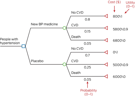
BP = blood pressure; CVD = cardiovascular disease.A simple decision tree constructed in TreeAge Pro. Blue box represents decision node, green circle represents chance node, red triangle represents terminal state. Example calculation of cost in the “New BP medicine” group: total cost (new BP medicine group) = 0.8*800 + 0.15*5800 + 0.05*6800 = $1850.

Box 5 – A Markov cohort model: new blood pressure medicine versus placebo

---

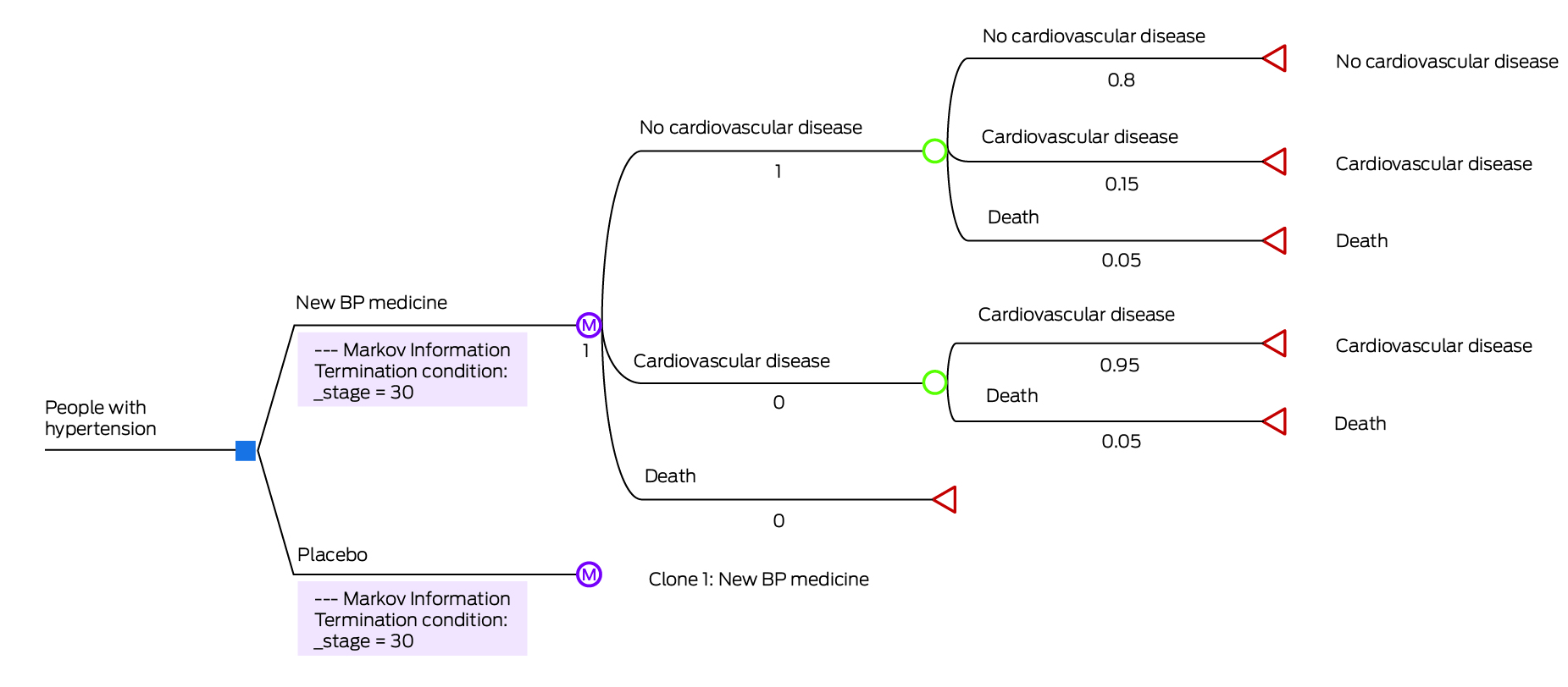
BP = blood pressure.A Markov model constructed in TreeAge Pro (simplified representation). Blue box represents decision node, purple circle represents Markov node, green circle represents chance node, red triangle represents terminal state.

Box 6 – Markov cohort versus Markov microsimulation – the first four cycles (years)

---

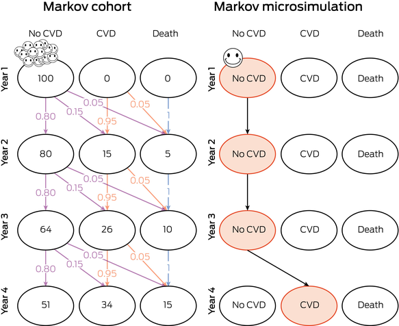
CVD = cardiovascular disease.Visual representation of Markov cohort (left) versus Markov microsimulation (right) in initial Years 1 to 4. In the Markov cohort model, the smiley faces represent the group of individuals moving through the model, according to probabilities of 0 to 1 (purple for probabilities from no CVD to other outcomes; orange for probabilities from CVD; blue for probabilities from death). The numbers within the bubbles represent the number of individuals in each health state at the end of each year. In the Markov microsimulation model, the smiley face represents a single individual moving through the model. The orange bubbles represent the pathway this individual takes through the simulation from Years 1 to 4. In the microsimulation, the individual simulations are repeated for a number of patients (eg, 100 individuals).

Box 7 – Example of probabilistic sensitivity analysis results (1000 runs) plotted on a cost‐effectiveness plane

---

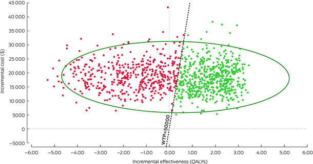
QALY = quality adjusted life years; WTP = willingness to pay (threshold).Generated in TreeAge Pro. The diagonal dotted line represents an arbitrary willingness to pay threshold of $50 000 per QALY. Red dots represent each run that is above the willingness to pay threshold (considered not cost‐effective), whereas green dots represent each run that is below the willingness to pay threshold (considered cost‐effective). The larger green circle represents a 95% confidence interval around the estimated ICER of $75 742 per QALY.